There are two main ways geospatial data are stored
- rasters, where each ‘pixel’ stores data values. This corresponds to files such as geotiffs.
- vectors, where information is stored more like a table form, and each row will have a ‘geometry’ field which stores information that allows you to recreate a geographical feature, such as a point , a polygon etc. It might also store the coordinate reference system so you can correctly place the shapes on a map
This set of notes corresponds to handling raster data. For this, we will make use of the rasterio library for manipulating the data, as well as pyproj for coordinate transforms.
(You can access a running version of this notebook on colab here)
Setup
For this demo, I will be using a population dataset from NASA “Gridded Population of the World, Version 4 (GPWv4): Population Count Adjusted to Match 2015 Revision of UN WPP Country Totals”
!pip install rasterio pyproj --quiet
import rasterio
import pyproj
import numpy as np
import pandas as pd
import matplotlib.pyplot as plt

%matplotlib inline
peak at data:
asc is much like a text file and we can use conventional text handling tools and a bit of pandas to parse it, but it is much less mistake prone if we use rasterio to handle it
!cat gpw_v4_population_count_adjusted_to_2015_unwpp_country_totals_rev11_2020_1_deg.asc | head -6
ncols         360
nrows         180
xllcorner     -180
yllcorner     -90
cellsize      1.0000000000001
NODATA_value  -9999
-9999 -9999 -9999 -9999 -9999 -9999 -9999 -9999 -9999 -9999 -9999 -9999 -9999 -9999 -9999 -9999 -9999 -9999 -9999 -9999 -9999 -9999 -9999 -9999 -9999 -9999 -9999 -9999 -9999 -9999 -9999 -9999 -9999 -9999
...
!cat gpw_v4_population_count_adjusted_to_2015_unwpp_country_totals_rev11_2020_1_deg.prj | head -10
Projection    GEOGRAPHIC
Datum         WGS84
Spheroid      WGS84
Units         DD
Zunits        NO
Parameters
parsing the data
For this example, we would like to convert the raster to a tabular form we can store in a ‘conventional’ database/csv file. For this, we will do these tasks:
read the file into memory
filter out any pixels/cells with no data
convert the data into a ’long’ table with the format
longitude | latitude | population |obtain the lat/lng values in web mercator coordinates
Read the file: note that rasterio can also open files on certain cloud providers, such as GCS/S3 etc, just pass it the relevant filepath in
gs://,s3://format
dataset = rasterio.open("gpw_v4_population_count_adjusted_to_2015_unwpp_country_totals_rev11_2020_1_deg.asc")
the dataset object holds metadata:
# extent of the data and crs -- note we are getting the CRS info from the .prj file also supplied
dataset.bounds, dataset.crs
(BoundingBox(left=-180.0, bottom=-90.0, right=180.0, top=90.0),
 CRS.from_epsg(4326))
The actual values of the pixels are in the 1st ‘band’. There can be more than 1 band– for example satellite imagery can comes in > 10 bands. We can either read all the bands in at once, or one by one. (Note that the indexing starts with 1 for the bands if reading in one by one)
data= dataset.read()
data.shape
(1, 180, 360)
# from the above, we know that there is only 1 band, so we can convert the data to a 2d array
data = data.squeeze()
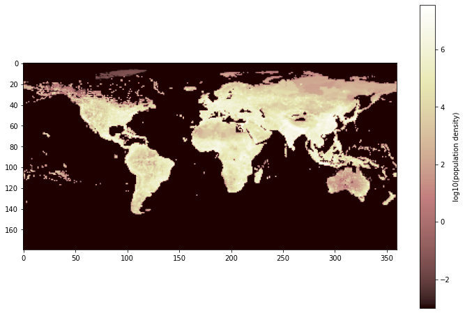
- remove all pixels with no data
valid_rows, valid_cols = np.nonzero(data != dataset.get_nodatavals())
valid_data_vals = data[(valid_rows, valid_cols)]
plt_data = np.zeros_like(data)
plt_data[(valid_rows, valid_cols)] = valid_data_vals

f, ax = plt.subplots(figsize=(12, 8))
ax1 = ax.imshow(np.log10(plt_data+0.001), cmap='pink')
f.colorbar(ax1, label=f"log10(population density)");
- Convert pixel positions to coordinates:
# covert rows, cols to coordinates:
valid_lngs, valid_lats = rasterio.transform.xy(dataset.transform, valid_rows, valid_cols)
output_dataframe = pd.DataFrame(
    data = dict(
        lat=valid_lats,
        lng = valid_lngs,
        population = valid_data_vals
    )
)
output_dataframe.sample(frac=1.).head()
| index | lat | lng | population |
|---|---|---|---|
| 6506 | 53.5 | 124.5 | 9.351563e+03 |
| 1035 | 75.5 | 141.5 | 1.780356e+02 |
| 3034 | 66.5 | 72.5 | 1.972377e+03 |
| 7488 | 48.5 | -113.5 | 9.566622e+03 |
| 10740 | 32.5 | 116.5 | 4.994749e+06 |
Add lat lng values in web mercator:
(note that it is a good idea to always_xy param to be true, this means the order of the output is always in the coordinates’ equivalent to longitude, latitude. There are CRS that can end up swapping the x, y axis from the source CRS)
dataset.crs
CRS.from_epsg(4326)
transformer = pyproj.Transformer.from_crs("EPSG:4326", "EPSG:3857", always_xy=True)
lng_3857, lat_3857 = transformer.transform(output_dataframe.lng.values.squeeze(), output_dataframe.lat.values.squeeze())

output_dataframe['lng_3857'] = lng_3857
output_dataframe['lat_3857'] = lat_3857
output_dataframe.sample(frac=1.).head()
| index | lat | lng | population | lng_3857 | lat_3857 |
|---|---|---|---|---|---|
| 11941 | 25.5 | 124.5 | 2.870859e+01 | 1.385928e+07 | 2.937284e+06 |
| 17692 | -22.5 | 117.5 | 4.557170e+03 | 1.308004e+07 | -2.571663e+06 |
| 44 | 82.5 | -77.5 | 3.311810e-02 | -8.627261e+06 | 1.738069e+07 |
| 9618 | 38.5 | 46.5 | 1.455383e+06 | 5.176356e+06 | 4.650302e+06 |
| 16594 | -12.5 | 122.5 | 1.345766e-03 | 1.363664e+07 | -1.402665e+06 |
# verify and sanity check
output_dataframe.isnull().sum()
lat           0
lng           0
population    0
lng_3857      0
lat_3857      0
dtype: int64